Chapter 5. Data transformation
R4DS github reference: r4ds/transform.Rmd
5.2 Filter rows with filter()
As a prerequisite install the tidyverse and nycflights13 packages.
if (!require("tidyverse")) install.packages("tidyverse")
library(tidyverse)
if (!require("nycflights13")) install.packages("nycflights13")
library(nycflights13)
Question 1: Find all flights that:
1) Had an arrival delay of two or more hours
2) Flew to Houston (IAH or HOU)
3) Were operated by United, American, or Delta
4) Departed in summer (July, August, and September)
5) Arrived more than two hours late, but didn’t leave late
6) Were delayed by at least an hour, but made up over 30 minutes in flight
7) Departed between midnight and 6am (inclusive)
Part 1) Pay attention to the fact that arr_delay is measured in minutes.
## # A tibble: 10,200 x 19
##     year month   day dep_time sched_dep_time dep_delay arr_time
##    <int> <int> <int>    <int>          <int>     <dbl>    <int>
##  1  2013     1     1      811            630       101     1047
##  2  2013     1     1      848           1835       853     1001
##  3  2013     1     1      957            733       144     1056
##  4  2013     1     1     1114            900       134     1447
##  5  2013     1     1     1505           1310       115     1638
##  6  2013     1     1     1525           1340       105     1831
##  7  2013     1     1     1549           1445        64     1912
##  8  2013     1     1     1558           1359       119     1718
##  9  2013     1     1     1732           1630        62     2028
## 10  2013     1     1     1803           1620       103     2008
## # ... with 10,190 more rows, and 12 more variables: sched_arr_time <int>,
## #   arr_delay <dbl>, carrier <chr>, flight <int>, tailnum <chr>,
## #   origin <chr>, dest <chr>, air_time <dbl>, distance <dbl>, hour <dbl>,
## #   minute <dbl>, time_hour <dttm>
Part 2)
## # A tibble: 9,313 x 19
##     year month   day dep_time sched_dep_time dep_delay arr_time
##    <int> <int> <int>    <int>          <int>     <dbl>    <int>
##  1  2013     1     1      517            515         2      830
##  2  2013     1     1      533            529         4      850
##  3  2013     1     1      623            627        -4      933
##  4  2013     1     1      728            732        -4     1041
##  5  2013     1     1      739            739         0     1104
##  6  2013     1     1      908            908         0     1228
##  7  2013     1     1     1028           1026         2     1350
##  8  2013     1     1     1044           1045        -1     1352
##  9  2013     1     1     1114            900       134     1447
## 10  2013     1     1     1205           1200         5     1503
## # ... with 9,303 more rows, and 12 more variables: sched_arr_time <int>,
## #   arr_delay <dbl>, carrier <chr>, flight <int>, tailnum <chr>,
## #   origin <chr>, dest <chr>, air_time <dbl>, distance <dbl>, hour <dbl>,
## #   minute <dbl>, time_hour <dttm>
Part 3)
## # A tibble: 139,504 x 19
##     year month   day dep_time sched_dep_time dep_delay arr_time
##    <int> <int> <int>    <int>          <int>     <dbl>    <int>
##  1  2013     1     1      517            515         2      830
##  2  2013     1     1      533            529         4      850
##  3  2013     1     1      542            540         2      923
##  4  2013     1     1      554            600        -6      812
##  5  2013     1     1      554            558        -4      740
##  6  2013     1     1      558            600        -2      753
##  7  2013     1     1      558            600        -2      924
##  8  2013     1     1      558            600        -2      923
##  9  2013     1     1      559            600        -1      941
## 10  2013     1     1      559            600        -1      854
## # ... with 139,494 more rows, and 12 more variables: sched_arr_time <int>,
## #   arr_delay <dbl>, carrier <chr>, flight <int>, tailnum <chr>,
## #   origin <chr>, dest <chr>, air_time <dbl>, distance <dbl>, hour <dbl>,
## #   minute <dbl>, time_hour <dttm>
Part 4)
## # A tibble: 86,326 x 19
##     year month   day dep_time sched_dep_time dep_delay arr_time
##    <int> <int> <int>    <int>          <int>     <dbl>    <int>
##  1  2013     7     1        1           2029       212      236
##  2  2013     7     1        2           2359         3      344
##  3  2013     7     1       29           2245       104      151
##  4  2013     7     1       43           2130       193      322
##  5  2013     7     1       44           2150       174      300
##  6  2013     7     1       46           2051       235      304
##  7  2013     7     1       48           2001       287      308
##  8  2013     7     1       58           2155       183      335
##  9  2013     7     1      100           2146       194      327
## 10  2013     7     1      100           2245       135      337
## # ... with 86,316 more rows, and 12 more variables: sched_arr_time <int>,
## #   arr_delay <dbl>, carrier <chr>, flight <int>, tailnum <chr>,
## #   origin <chr>, dest <chr>, air_time <dbl>, distance <dbl>, hour <dbl>,
## #   minute <dbl>, time_hour <dttm>
Part 5) Again arr_delay and dep_delay are measured in minutes.
## # A tibble: 29 x 19
##     year month   day dep_time sched_dep_time dep_delay arr_time
##    <int> <int> <int>    <int>          <int>     <dbl>    <int>
##  1  2013     1    27     1419           1420        -1     1754
##  2  2013    10     7     1350           1350         0     1736
##  3  2013    10     7     1357           1359        -2     1858
##  4  2013    10    16      657            700        -3     1258
##  5  2013    11     1      658            700        -2     1329
##  6  2013     3    18     1844           1847        -3       39
##  7  2013     4    17     1635           1640        -5     2049
##  8  2013     4    18      558            600        -2     1149
##  9  2013     4    18      655            700        -5     1213
## 10  2013     5    22     1827           1830        -3     2217
## # ... with 19 more rows, and 12 more variables: sched_arr_time <int>,
## #   arr_delay <dbl>, carrier <chr>, flight <int>, tailnum <chr>,
## #   origin <chr>, dest <chr>, air_time <dbl>, distance <dbl>, hour <dbl>,
## #   minute <dbl>, time_hour <dttm>
Part 6) Making up over 30 minutes during flight, means that with respect of dep_delay the arr_delay is at least 30 minutes less, therefore arr_delay < dep_delay - 30.
## # A tibble: 1,844 x 19
##     year month   day dep_time sched_dep_time dep_delay arr_time
##    <int> <int> <int>    <int>          <int>     <dbl>    <int>
##  1  2013     1     1     2205           1720       285       46
##  2  2013     1     1     2326           2130       116      131
##  3  2013     1     3     1503           1221       162     1803
##  4  2013     1     3     1839           1700        99     2056
##  5  2013     1     3     1850           1745        65     2148
##  6  2013     1     3     1941           1759       102     2246
##  7  2013     1     3     1950           1845        65     2228
##  8  2013     1     3     2015           1915        60     2135
##  9  2013     1     3     2257           2000       177       45
## 10  2013     1     4     1917           1700       137     2135
## # ... with 1,834 more rows, and 12 more variables: sched_arr_time <int>,
## #   arr_delay <dbl>, carrier <chr>, flight <int>, tailnum <chr>,
## #   origin <chr>, dest <chr>, air_time <dbl>, distance <dbl>, hour <dbl>,
## #   minute <dbl>, time_hour <dttm>
Part 7) Pay attention to the fact that midnight is represented by 2400 and not 0.
## # A tibble: 9,373 x 19
##     year month   day dep_time sched_dep_time dep_delay arr_time
##    <int> <int> <int>    <int>          <int>     <dbl>    <int>
##  1  2013     1     1      517            515         2      830
##  2  2013     1     1      533            529         4      850
##  3  2013     1     1      542            540         2      923
##  4  2013     1     1      544            545        -1     1004
##  5  2013     1     1      554            600        -6      812
##  6  2013     1     1      554            558        -4      740
##  7  2013     1     1      555            600        -5      913
##  8  2013     1     1      557            600        -3      709
##  9  2013     1     1      557            600        -3      838
## 10  2013     1     1      558            600        -2      753
## # ... with 9,363 more rows, and 12 more variables: sched_arr_time <int>,
## #   arr_delay <dbl>, carrier <chr>, flight <int>, tailnum <chr>,
## #   origin <chr>, dest <chr>, air_time <dbl>, distance <dbl>, hour <dbl>,
## #   minute <dbl>, time_hour <dttm>
Question 2: Another useful dplyr filtering helper is between(). What does it do? Can you use it to simplify the code needed to answer the previous challenges?
between() helper is a shortcut for x >= left & x <= right. For instance for Part 4 of previous question we could have used:
## # A tibble: 86,326 x 19
##     year month   day dep_time sched_dep_time dep_delay arr_time
##    <int> <int> <int>    <int>          <int>     <dbl>    <int>
##  1  2013     7     1        1           2029       212      236
##  2  2013     7     1        2           2359         3      344
##  3  2013     7     1       29           2245       104      151
##  4  2013     7     1       43           2130       193      322
##  5  2013     7     1       44           2150       174      300
##  6  2013     7     1       46           2051       235      304
##  7  2013     7     1       48           2001       287      308
##  8  2013     7     1       58           2155       183      335
##  9  2013     7     1      100           2146       194      327
## 10  2013     7     1      100           2245       135      337
## # ... with 86,316 more rows, and 12 more variables: sched_arr_time <int>,
## #   arr_delay <dbl>, carrier <chr>, flight <int>, tailnum <chr>,
## #   origin <chr>, dest <chr>, air_time <dbl>, distance <dbl>, hour <dbl>,
## #   minute <dbl>, time_hour <dttm>
Question 3: How many flights have a missing dep_time? What other variables are missing? What might these rows represent?
We can use the is.na function:
## # A tibble: 8,255 x 19
##     year month   day dep_time sched_dep_time dep_delay arr_time
##    <int> <int> <int>    <int>          <int>     <dbl>    <int>
##  1  2013     1     1       NA           1630        NA       NA
##  2  2013     1     1       NA           1935        NA       NA
##  3  2013     1     1       NA           1500        NA       NA
##  4  2013     1     1       NA            600        NA       NA
##  5  2013     1     2       NA           1540        NA       NA
##  6  2013     1     2       NA           1620        NA       NA
##  7  2013     1     2       NA           1355        NA       NA
##  8  2013     1     2       NA           1420        NA       NA
##  9  2013     1     2       NA           1321        NA       NA
## 10  2013     1     2       NA           1545        NA       NA
## # ... with 8,245 more rows, and 12 more variables: sched_arr_time <int>,
## #   arr_delay <dbl>, carrier <chr>, flight <int>, tailnum <chr>,
## #   origin <chr>, dest <chr>, air_time <dbl>, distance <dbl>, hour <dbl>,
## #   minute <dbl>, time_hour <dttm>
8255 rows show a missing dep_time as well as a missing arr_time. Probably they are cancelled flights.
Question 4: Why is NA ^ 0 not missing? Why is NA | TRUE not missing? Why is FALSE & NA not missing? Can you figure out the general rule? ( NA * 0 is a tricky counterexample!)
NA ^ 0 is equal to 1, as every number raised to the 0th power is 1. NA | TRUE is true, as logical or expression with a true term is always true. Similarly FALSE & NA is false, as logical and expression with a false term is always false. Finally NA * 0 is not defined since arithmetic operators in an NA expression lead to a not a number result.
Here’s tha calculated expressions:
## [1] 1## [1] TRUE## [1] FALSE## [1] NA## [1] NA5.3 Arrange rows with arrange()
Question 1: How could you use arrange() to sort all missing values to the start? (Hint: use is.na()).
Since the missing values are always sorted at the end, despite the use of the desc function, we can use the is.na function to specify a vector of booleans and then apply the desc function. Let’s consider the dep_time column:
## # A tibble: 336,776 x 19
##     year month   day dep_time sched_dep_time dep_delay arr_time
##    <int> <int> <int>    <int>          <int>     <dbl>    <int>
##  1  2013     1     1       NA           1630        NA       NA
##  2  2013     1     1       NA           1935        NA       NA
##  3  2013     1     1       NA           1500        NA       NA
##  4  2013     1     1       NA            600        NA       NA
##  5  2013     1     2       NA           1540        NA       NA
##  6  2013     1     2       NA           1620        NA       NA
##  7  2013     1     2       NA           1355        NA       NA
##  8  2013     1     2       NA           1420        NA       NA
##  9  2013     1     2       NA           1321        NA       NA
## 10  2013     1     2       NA           1545        NA       NA
## # ... with 336,766 more rows, and 12 more variables: sched_arr_time <int>,
## #   arr_delay <dbl>, carrier <chr>, flight <int>, tailnum <chr>,
## #   origin <chr>, dest <chr>, air_time <dbl>, distance <dbl>, hour <dbl>,
## #   minute <dbl>, time_hour <dttm>
As a check we can look at the last few values:
## # A tibble: 6 x 19
##    year month   day dep_time sched_dep_time dep_delay arr_time
##   <int> <int> <int>    <int>          <int>     <dbl>    <int>
## 1  2013     9    30     2237           2245        -8     2345
## 2  2013     9    30     2240           2245        -5     2334
## 3  2013     9    30     2240           2250       -10     2347
## 4  2013     9    30     2241           2246        -5     2345
## 5  2013     9    30     2307           2255        12     2359
## 6  2013     9    30     2349           2359       -10      325
## # ... with 12 more variables: sched_arr_time <int>, arr_delay <dbl>,
## #   carrier <chr>, flight <int>, tailnum <chr>, origin <chr>, dest <chr>,
## #   air_time <dbl>, distance <dbl>, hour <dbl>, minute <dbl>,
## #   time_hour <dttm>
Question 2: Sort flights to find the most delayed flights. Find the flights that left earliest.
From the documentation we know that dep_delay and arr_delay are departure and arrival delays, in minutes. And that negative times represent early departures/arrivals. We can build a total delay value by summing these two values and sort the dataframe accordingly.
## # A tibble: 336,776 x 19
##     year month   day dep_time sched_dep_time dep_delay arr_time
##    <int> <int> <int>    <int>          <int>     <dbl>    <int>
##  1  2013     1     9      641            900      1301     1242
##  2  2013     6    15     1432           1935      1137     1607
##  3  2013     1    10     1121           1635      1126     1239
##  4  2013     9    20     1139           1845      1014     1457
##  5  2013     7    22      845           1600      1005     1044
##  6  2013     4    10     1100           1900       960     1342
##  7  2013     3    17     2321            810       911      135
##  8  2013     7    22     2257            759       898      121
##  9  2013    12     5      756           1700       896     1058
## 10  2013     5     3     1133           2055       878     1250
## # ... with 336,766 more rows, and 12 more variables: sched_arr_time <int>,
## #   arr_delay <dbl>, carrier <chr>, flight <int>, tailnum <chr>,
## #   origin <chr>, dest <chr>, air_time <dbl>, distance <dbl>, hour <dbl>,
## #   minute <dbl>, time_hour <dttm>
By sorting in ascending order on the dep_delay we’re then able to see the flights that left earlier:
## # A tibble: 336,776 x 19
##     year month   day dep_time sched_dep_time dep_delay arr_time
##    <int> <int> <int>    <int>          <int>     <dbl>    <int>
##  1  2013    12     7     2040           2123       -43       40
##  2  2013     2     3     2022           2055       -33     2240
##  3  2013    11    10     1408           1440       -32     1549
##  4  2013     1    11     1900           1930       -30     2233
##  5  2013     1    29     1703           1730       -27     1947
##  6  2013     8     9      729            755       -26     1002
##  7  2013    10    23     1907           1932       -25     2143
##  8  2013     3    30     2030           2055       -25     2213
##  9  2013     3     2     1431           1455       -24     1601
## 10  2013     5     5      934            958       -24     1225
## # ... with 336,766 more rows, and 12 more variables: sched_arr_time <int>,
## #   arr_delay <dbl>, carrier <chr>, flight <int>, tailnum <chr>,
## #   origin <chr>, dest <chr>, air_time <dbl>, distance <dbl>, hour <dbl>,
## #   minute <dbl>, time_hour <dttm>
Question 3: Sort flights to find the fastest (highest speed) flights.
To simplify the exercise we can consider the average speed as: distance / air_time and sort by this calculated value.
To obtain a miles/hours speed we should divide the air_time by 60.
## # A tibble: 336,776 x 19
##     year month   day dep_time sched_dep_time dep_delay arr_time
##    <int> <int> <int>    <int>          <int>     <dbl>    <int>
##  1  2013     5    25     1709           1700         9     1923
##  2  2013     7     2     1558           1513        45     1745
##  3  2013     5    13     2040           2025        15     2225
##  4  2013     3    23     1914           1910         4     2045
##  5  2013     1    12     1559           1600        -1     1849
##  6  2013    11    17      650            655        -5     1059
##  7  2013     2    21     2355           2358        -3      412
##  8  2013    11    17      759            800        -1     1212
##  9  2013    11    16     2003           1925        38       17
## 10  2013    11    16     2349           2359       -10      402
## # ... with 336,766 more rows, and 12 more variables: sched_arr_time <int>,
## #   arr_delay <dbl>, carrier <chr>, flight <int>, tailnum <chr>,
## #   origin <chr>, dest <chr>, air_time <dbl>, distance <dbl>, hour <dbl>,
## #   minute <dbl>, time_hour <dttm>
Question 4: Which flights travelled the farthest? Which travelled the shortest?
We can simply sort on the distance field. For the farthest in descending order and ascending in the shortest.
## # A tibble: 336,776 x 19
##     year month   day dep_time sched_dep_time dep_delay arr_time
##    <int> <int> <int>    <int>          <int>     <dbl>    <int>
##  1  2013     1     1      857            900        -3     1516
##  2  2013     1     2      909            900         9     1525
##  3  2013     1     3      914            900        14     1504
##  4  2013     1     4      900            900         0     1516
##  5  2013     1     5      858            900        -2     1519
##  6  2013     1     6     1019            900        79     1558
##  7  2013     1     7     1042            900       102     1620
##  8  2013     1     8      901            900         1     1504
##  9  2013     1     9      641            900      1301     1242
## 10  2013     1    10      859            900        -1     1449
## # ... with 336,766 more rows, and 12 more variables: sched_arr_time <int>,
## #   arr_delay <dbl>, carrier <chr>, flight <int>, tailnum <chr>,
## #   origin <chr>, dest <chr>, air_time <dbl>, distance <dbl>, hour <dbl>,
## # minute <dbl>, time_hour <dttm>## # A tibble: 336,776 x 19
## year month day dep_time sched_dep_time dep_delay arr_time
## <int> <int> <int> <int> <int> <dbl> <int>
## 1 2013 7 27 NA 106 NA NA
## 2 2013 1 3 2127 2129 -2 2222
## 3 2013 1 4 1240 1200 40 1333
## 4 2013 1 4 1829 1615 134 1937
## 5 2013 1 4 2128 2129 -1 2218
## 6 2013 1 5 1155 1200 -5 1241
## 7 2013 1 6 2125 2129 -4 2224
## 8 2013 1 7 2124 2129 -5 2212
## 9 2013 1 8 2127 2130 -3 2304
## 10 2013 1 9 2126 2129 -3 2217
## # ... with 336,766 more rows, and 12 more variables: sched_arr_time <int>,
## # arr_delay <dbl>, carrier <chr>, flight <int>, tailnum <chr>,
## # origin <chr>, dest <chr>, air_time <dbl>, distance <dbl>, hour <dbl>,
## # minute <dbl>, time_hour <dttm>5.4 Select columns with select()
Question 1: Brainstorm as many ways as possible to select dep_time, dep_delay, arr_time, and arr_delay from flights.
Examples of selection can be made by:
- specifying columns name:
## # A tibble: 336,776 x 4
##    dep_time dep_delay arr_time arr_delay
##       <int>     <dbl>    <int>     <dbl>
##  1      517         2      830        11
##  2      533         4      850        20
##  3      542         2      923        33
##  4      544        -1     1004       -18
##  5      554        -6      812       -25
##  6      554        -4      740        12
##  7      555        -5      913        19
##  8      557        -3      709       -14
##  9      557        -3      838        -8
## 10      558        -2      753         8
## # ... with 336,766 more rows- specifying columns position:
## # A tibble: 336,776 x 4
##    dep_time dep_delay arr_time arr_delay
##       <int>     <dbl>    <int>     <dbl>
##  1      517         2      830        11
##  2      533         4      850        20
##  3      542         2      923        33
##  4      544        -1     1004       -18
##  5      554        -6      812       -25
##  6      554        -4      740        12
##  7      555        -5      913        19
##  8      557        -3      709       -14
##  9      557        -3      838        -8
## 10      558        -2      753         8
## # ... with 336,766 more rows- using the
starts_withhelper:
## # A tibble: 336,776 x 4
##    dep_time dep_delay arr_time arr_delay
##       <int>     <dbl>    <int>     <dbl>
##  1      517         2      830        11
##  2      533         4      850        20
##  3      542         2      923        33
##  4      544        -1     1004       -18
##  5      554        -6      812       -25
##  6      554        -4      740        12
##  7      555        -5      913        19
##  8      557        -3      709       -14
##  9      557        -3      838        -8
## 10      558        -2      753         8
## # ... with 336,766 more rows
Question 2: What happens if you include the name of a variable multiple times in a select() call?
The select statement takes each variable only one time and therefore it won’t be affected by duplications.
## # A tibble: 336,776 x 3
##    dep_time arr_time arr_delay
##       <int>    <int>     <dbl>
##  1      517      830        11
##  2      533      850        20
##  3      542      923        33
##  4      544     1004       -18
##  5      554      812       -25
##  6      554      740        12
##  7      555      913        19
##  8      557      709       -14
##  9      557      838        -8
## 10      558      753         8
## # ... with 336,766 more rows
Question 3: What does the one_of() function do? Why might it be helpful in conjunction with this vector? vars <- c("year", "month", "day", "dep_delay", "arr_delay")
one_of() helper can be used, once we define a vector of names, to make more readable the select statement. It can be used as another way to select columns (see question 1).
## # A tibble: 336,776 x 5
##     year month   day dep_delay arr_delay
##    <int> <int> <int>     <dbl>     <dbl>
##  1  2013     1     1         2        11
##  2  2013     1     1         4        20
##  3  2013     1     1         2        33
##  4  2013     1     1        -1       -18
##  5  2013     1     1        -6       -25
##  6  2013     1     1        -4        12
##  7  2013     1     1        -5        19
##  8  2013     1     1        -3       -14
##  9  2013     1     1        -3        -8
## 10  2013     1     1        -2         8
## # ... with 336,766 more rows
Question 4: Does the result of running the following code surprise you? How do the select helpers deal with case by default? How can you change that default? select(flights, contains("TIME"))
The contains helper is case insensitive. It can be made case sensitive with the ignore.case = FALSE option.
## # A tibble: 336,776 x 6
##    dep_time sched_dep_time arr_time sched_arr_time air_time
##       <int>          <int>    <int>          <int>    <dbl>
##  1      517            515      830            819      227
##  2      533            529      850            830      227
##  3      542            540      923            850      160
##  4      544            545     1004           1022      183
##  5      554            600      812            837      116
##  6      554            558      740            728      150
##  7      555            600      913            854      158
##  8      557            600      709            723       53
##  9      557            600      838            846      140
## 10      558            600      753            745      138
## # ... with 336,766 more rows, and 1 more variable: time_hour <dttm>## # A tibble: 336,776 x 05.5 Add new variables with mutate()
Question 1: Currently dep_time and sched_dep_time are convenient to look at, but hard to compute with because they’re not really continuous numbers. Convert them to a more convenient representation of number of minutes since midnight.
Starting from the example in the book we can extract the hours and minutes of both fields with the following statements:
hours = dep_time %/% 100minutes = dep_time %% 100
Then we get the total minutes by summing up hours*60 + minutes. Finally we can extract only the columns we’re interesed in.
select(
  mutate(flights,
       dep_time_minutes = (dep_time %/% 100)*60 + dep_time %% 100,
       sched_dep_time_minutes = (sched_dep_time %/% 100)*60 + sched_dep_time %% 100
  ),
  dep_time, sched_dep_time,
  dep_time_minutes, sched_dep_time_minutes
)
## # A tibble: 336,776 x 4
## dep_time sched_dep_time dep_time_minutes sched_dep_time_minutes
## <int> <int> <dbl> <dbl>
## 1 517 515 317 315
## 2 533 529 333 329
## 3 542 540 342 340
## 4 544 545 344 345
## 5 554 600 354 360
## 6 554 558 354 358
## 7 555 600 355 360
## 8 557 600 357 360
## 9 557 600 357 360
## 10 558 600 358 360
## # ... with 336,766 more rows
Question 2: Compare air_time with arr_time - dep_time. What do you expect to see? What do you see? What do you need to do to fix it?
From the documentation the hypothesis is that the air_time = arr_time - dep_time.
To test the hypothesis we should first create a new dataframe by converting the value in minutes. We can use the previous solution.
flights_diff <- mutate(flights,
       dep_time_minutes = (dep_time %/% 100)*60 + dep_time %% 100,
       arr_time_minutes = (arr_time %/% 100)*60 + arr_time %% 100,
       delta = arr_time_minutes - dep_time_minutes
)


nrow(filter(flights_diff, air_time != delta))/nrow(flights)*100
## [1] 97.14172We can see that for roughly 97% of the records the equality is not satisfied. By looking at the documentation we see that the fields involved are defined as:
dep_time,arr_timeActual departure and arrival times (format HHMM or HMM), local tzair_timeAmount of time spent in the air, in minutes
One possibile reason of such number of non equal record can be the fact that air_time doesn’t count the time needed by the aircraft to go in the air (takeoff and landing for instance).
But this may not be the only reason since if we compute the records where air_time < delta (the air_time lacks always a certain amount of time - takeoff and landing - so we can suppose that it would be less than delta), we find that this explains only 58% of the records with inequality.
## [1] 0.5804157
Question 3: Compare dep_time, sched_dep_time, and dep_delay. How would you expect those three numbers to be related?
sched_dep_time should be the scheduled departure time of the flight while dep_time should be the effective departure time. The difference between the two is the departure delay: dep_delay. So the relationship should be dep_delay = sched_dep_time - dep_time.
As done in the previous question we can have a check of the hypothesis by doing a bit of conversions:
flights_diff2 <- mutate(flights,
       sched_dep_time_minutes = (sched_dep_time %/% 100)*60 + sched_dep_time %% 100,
       dep_time_minutes = (dep_time %/% 100)*60 + dep_time %% 100,
       delta = sched_dep_time_minutes - dep_time_minutes
)


nrow(filter(flights_diff2, dep_delay != delta))/nrow(flights)*100
## [1] 92.64526In this case again the majority of the records do not satisfy the hypothesis. Probably some element in the collection of the data may explain that.
Question 4: Find the 10 most delayed flights using a ranking function. How do you want to handle ties? Carefully read the documentation for min_rank()
From the question 2 of the §5.3 we can create calculate the total delay from the sum of dep_delay + arr_delay. By sorting in descending order, selecting a subset of fields and extracting the first 10 records we obtain:
head(
    select(
      arrange(mutate(flights, total_delay = dep_delay + arr_delay), desc(total_delay)),
      total_delay, carrier, flight, origin, dest, time_hour
    ),
    10
)
## # A tibble: 10 x 6
## total_delay carrier flight origin dest time_hour
## <dbl> <chr> <int> <chr> <chr> <dttm>
## 1 2573 HA 51 JFK HNL 2013-01-09 09:00:00
## 2 2264 MQ 3535 JFK CMH 2013-06-15 19:00:00
## 3 2235 MQ 3695 EWR ORD 2013-01-10 16:00:00
## 4 2021 AA 177 JFK SFO 2013-09-20 18:00:00
## 5 1994 MQ 3075 JFK CVG 2013-07-22 16:00:00
## 6 1891 DL 2391 JFK TPA 2013-04-10 19:00:00
## 7 1826 DL 2119 LGA MSP 2013-03-17 08:00:00
## 8 1793 DL 2047 LGA ATL 2013-07-22 07:00:00
## 9 1774 AA 172 EWR MIA 2013-12-05 17:00:00
## 10 1753 MQ 3744 EWR ORD 2013-05-03 20:00:00By looking at the results there is no need of additional sorting function (no ties). In case of ties dplyr has the following ranking functions If min_rank() doesn’t do what you need, look at the variants row_number(), dense_rank(), percent_rank(), cume_dist(), ntile().
5.6 Grouped summaries with summarise()
Question 1: Brainstorm at least 5 different ways to assess the typical delay characteristics of a group of flights. Consider the following scenarios:
1) A flight is 15 minutes early 50% of the time, and 15 minutes late 50% of the time.
2) A flight is always 10 minutes late.
3) A flight is 30 minutes early 50% of the time, and 30 minutes late 50% of the time.
4) 99% of the time a flight is on time. 1% of the time it’s 2 hours late.
5) Which is more important: arrival delay or departure delay?
Probably the answer depends of the trade-off. There are situations and customers where the delay is costly at the arrival and others where it is costly at the departure (eg. connections of multi flights for one trip).
Question 2: Come up with another approach that will give you the same output as not_cancelled %>% count(dest) and not_cancelled %>% count(tailnum, wt = distance) (without using count()).
Recall that:
We can use group_by and summarise. Then we specify the number of occurence with n() and the sum of distance with sum().
## # A tibble: 104 x 2
##    dest  `n()`
##    <chr> <int>
##  1 ABQ     254
##  2 ACK     264
##  3 ALB     418
##  4 ANC       8
##  5 ATL   16837
##  6 AUS    2411
##  7 AVL     261
##  8 BDL     412
##  9 BGR     358
## 10 BHM     269
## # ... with 94 more rows## # A tibble: 4,037 x 2
## tailnum `sum(distance)`
## <chr> <dbl>
## 1 D942DN 3418
## 2 N0EGMQ 239143
## 3 N10156 109664
## 4 N102UW 25722
## 5 N103US 24619
## 6 N104UW 24616
## 7 N10575 139903
## 8 N105UW 23618
## 9 N107US 21677
## 10 N108UW 32070
## # ... with 4,027 more rows
Question 3: Our definition of cancelled flights (is.na(dep_delay) | is.na(arr_delay) ) is slightly suboptimal. Why? Which is the most important column?
Probably the most important field is dep_delay. With a non NA value we know that a flight is scheduled, even if not on time.
Question 4: Look at the number of cancelled flights per day. Is there a pattern? Is the proportion of cancelled flights related to the average delay?
At first we can create a new dataframe with the total_delay and date fields, and then a filtered dataframe with the cancelled flights.
flights_grouped <- select(
  arrange(mutate(flights, total_delay = dep_delay + arr_delay, date = as.Date(format(time_hour, "%Y-%m-%d"))), desc(total_delay)),
  total_delay, dep_delay, arr_delay, carrier, flight, origin, dest, date
)

flights_grouped_cancelled <- flights_grouped %>% filter(is.na(dep_delay), is.na(arr_delay))
From this dataframe we can summarise the number of cancelled flights per day.
## # A tibble: 358 x 2
##    date       `n()`
##    <date>     <int>
##  1 2013-02-08   472
##  2 2013-02-09   393
##  3 2013-05-23   221
##  4 2013-12-10   204
##  5 2013-09-12   192
##  6 2013-03-06   180
##  7 2013-03-08   180
##  8 2013-12-05   158
##  9 2013-12-14   125
## 10 2013-06-28   123
## # ... with 348 more rows
We can also summarise the average daily delay.
flights_grouped %>% filter(!is.na(dep_delay), !is.na(arr_delay)) %>% group_by(date) %>%
  summarise(mean(total_delay)) %>% arrange(desc(`mean(total_delay)`))
## # A tibble: 365 x 2
## date `mean(total_delay)`
## <date> <dbl>
## 1 2013-03-08 170.
## 2 2013-07-01 115.
## 3 2013-05-23 113.
## 4 2013-07-10 111.
## 5 2013-07-22 109.
## 6 2013-06-13 109.
## 7 2013-09-12 108.
## 8 2013-12-05 104.
## 9 2013-06-24 98.7
## 10 2013-08-08 98.7
## # ... with 355 more rowsIt seems that in days where there are an high number of cancelled flights, there is corresponding high average daily delay. We can render it visually the previous two dataframes:
ggplot(data = flights_grouped_cancelled %>% group_by(date) %>% summarise(n()) %>% arrange(desc(`n()`))) +
  geom_line(aes(x=date, y=`n()`, group = 1))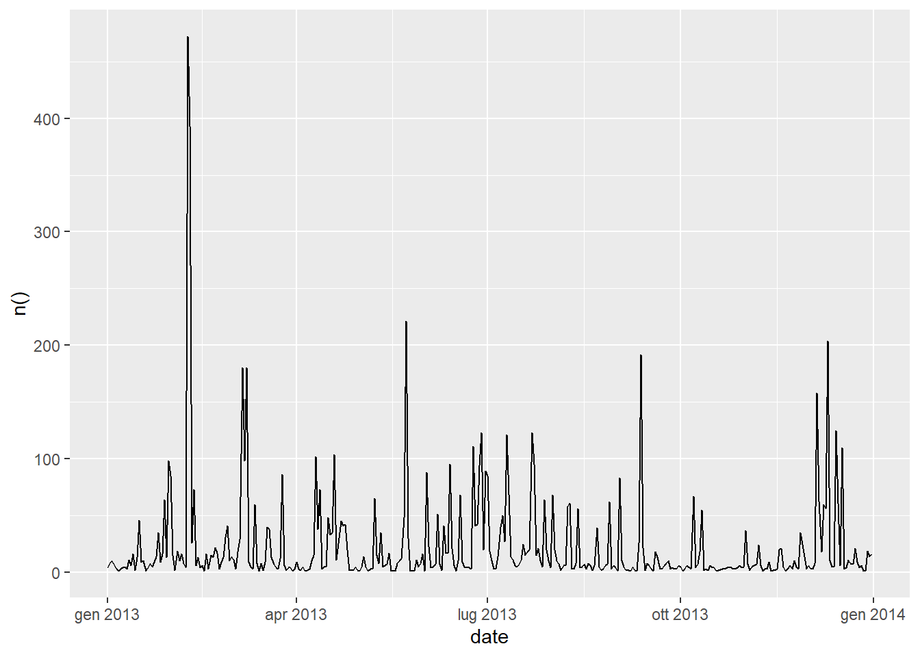
ggplot(data = flights_grouped %>% filter(!is.na(dep_delay), !is.na(arr_delay)) %>% group_by(date) %>%
  summarise(mean(total_delay)) %>% arrange(desc(`mean(total_delay)`))) +
  geom_line(aes(x=date, y=`mean(total_delay)`, group = 1))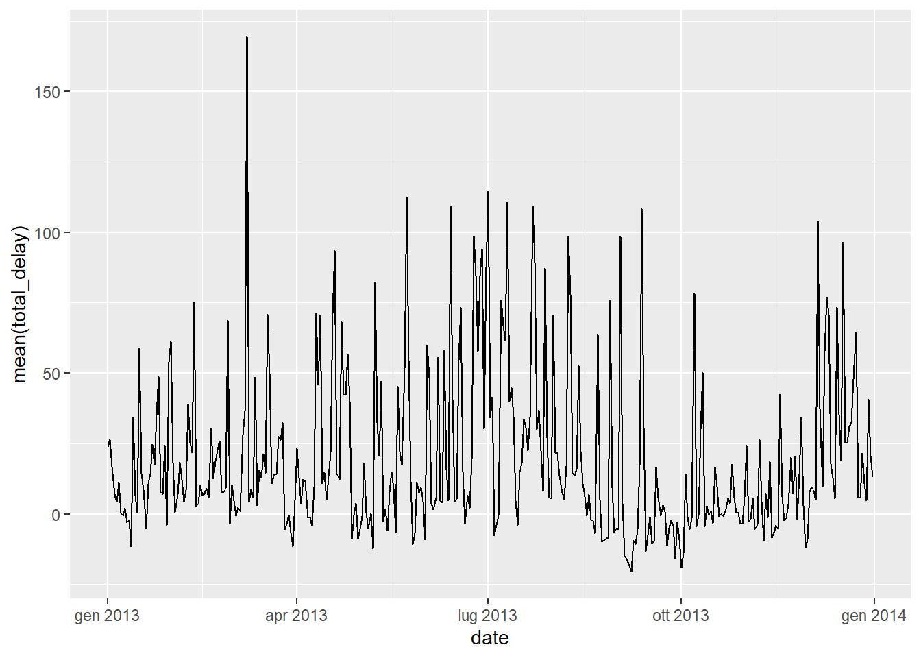
Question 5: Which carrier has the worst delays? Challenge: can you disentangle the effects of bad airports vs. bad carriers? Why/why not? (Hint: think about flights %>% group_by(carrier, dest) %>% summarise(n()))
The worst carrier is the one under the code B6 with a total delay in 2013 of 4603 minutes (over 76 hours!).
## # A tibble: 314 x 3
## # Groups:   carrier [16]
##    carrier dest  `sum(total_delay)`
##    <chr>   <chr>              <dbl>
##  1 B6      ABQ                 4603
##  2 MQ      TVC                  880
##  3 EV      PBI                  536
##  4 UA      STL                  375
##  5 EV      SBN                  276
##  6 OO      DTW                  259
##  7 OO      ORD                  174
##  8 DL      EYW                  170
##  9 UA      RDU                  116
## 10 UA      ANC                   83
## # ... with 304 more rows
This code corresponds to “JetBlue Airways” (seems that they suffer delays: https://fortune.com/2017/12/30/jetblue-flight-delays/).
## # A tibble: 1 x 2
##   carrier name
##   <chr>   <chr>
## 1 B6      JetBlue Airways
A possible way to disentangle the effects of bad airports versus bad carriers could be extract every possible route (fields origin and dest) and calculate the average delay for that route for each a carrier.
Question 6: What does the sort argument to count() do. When might you use it?
By looking at the help documentation the sort argument in the count() statement, when set to TRUE will sort output in descending order of n.
## # A tibble: 3,267 x 3
## # Groups:   carrier [16]
##    carrier air_time     n
##    <chr>      <dbl> <int>
##  1 9E            21     1
##  2 9E            22     1
##  3 9E            23    10
##  4 9E            24    25
##  5 9E            25    53
##  6 9E            26   100
##  7 9E            27   100
##  8 9E            28    83
##  9 9E            29    74
## 10 9E            30    54
## # ... with 3,257 more rows## # A tibble: 3,267 x 3
## # Groups: carrier [16]
## carrier air_time n
## <chr> <dbl> <int>
## 1 EV NA 3065
## 2 MQ NA 1360
## 3 9E NA 1166
## 4 EV 47 934
## 5 UA NA 883
## 6 EV 48 878
## 7 EV 46 862
## 8 EV 45 843
## 9 EV 49 834
## 10 AA NA 782
## # ... with 3,257 more rows5.7 Grouped mutates (and filters)
Question 1: Refer back to the lists of useful mutate and filtering functions. Describe how each operation changes when you combine it with grouping.
The difference lies in the way each function is being applied in each group. Let’s consider a filtered dataframe of the flights with tailnum equal to N153DL or N319AS and let’s extract the tailnum and air_time fields.
Let’s then create a new column which calculates the airtime mean then group by tailnum and again create a new column with airtime mean.
## # A tibble: 7 x 4
## # Groups:   tailnum [2]
##   tailnum air_time ungrouped_mean grouped_mean
##   <chr>      <dbl>          <dbl>        <dbl>
## 1 N319AS       328           266.         332.
## 2 N319AS       318           266.         332.
## 3 N319AS       349           266.         332.
## 4 N153DL       327           266.         216.
## 5 N153DL       118           266.         216.
## 6 N153DL       319           266.         216.
## 7 N153DL       102           266.         216.
We can see that the ungrouped_mean is calculated by considering all the air_time values as expexted since we calculated it before the group operation. But we can also see that the grouped_mean is calculated by considering all the air_time values with respect to their group:
ungrouped_mean= (328+318+349+327+118+319+102) /7=1861/7=265,857≃266grouped_mean= (328+318+349) /3=995/3=331,666≃332and (327+118+319+102) /4=216,5≃216
The mean() is an example of function who is being applied in each group.
Let’s now consider the arithmetic operator +. Let’s consider a new column which increments the airtime value by 100 before grouping and after grouping by tailnum as done before.
## # A tibble: 7 x 4
## # Groups:   tailnum [2]
##   tailnum air_time ungrouped_100_add grouped_100_add
##   <chr>      <dbl>             <dbl>           <dbl>
## 1 N319AS       328               428             428
## 2 N319AS       318               418             418
## 3 N319AS       349               449             449
## 4 N153DL       327               427             427
## 5 N153DL       118               218             218
## 6 N153DL       319               419             419
## 7 N153DL       102               202             202
We can see that the two columns have the same values: the arithmetic operator + is NOT an example of function who is being applied in each group.
In the same way we can test other functions.
Question 2: Which plane (tailnum) has the worst on-time record?
As the on-time record lets consider for semplicity the arr_delay field, that expresses the arrival delay of a flight in minutes. We suppose that this measure the quantity of time before/after the scheduled arrive time that a flight has. The plane with the worst value can be found with:
arrange(
  select(filter(flights, !is.na(arr_delay)), tailnum, arr_delay) %>% group_by(tailnum) %>% summarise(sum(arr_delay)),
  desc(`sum(arr_delay)`)
)
## # A tibble: 4,037 x 2
## tailnum `sum(arr_delay)`
## <chr> <dbl>
## 1 N15910 7317
## 2 N15980 7134
## 3 N16919 6904
## 4 N228JB 6778
## 5 N14998 6087
## 6 N192JB 5810
## 7 N292JB 5804
## 8 N12921 5788
## 9 N13958 5620
## 10 N10575 5566
## # ... with 4,027 more rowsWe selected all the flights with a non NA arr_delay and then grouping them by arr_delay. Sorting by the sum of arrival delays we obtain the tailnum N15910.
Question 3: What time of day should you fly if you want to avoid delays as much as possible?
We can basically apply the same piece of code of the previous question, only we substitute tailnum with hour. The top rows are the hours that register lower delays.
arrange(
  select(filter(flights, !is.na(arr_delay)), hour, arr_delay) %>% group_by(hour) %>% summarise(sum(arr_delay)),
  `sum(arr_delay)`
)
## # A tibble: 19 x 2
## hour `sum(arr_delay)`
## <dbl> <dbl>
## 1 7 -119218
## 2 6 -86125
## 3 8 -29761
## 4 9 -28928
## 5 5 -9306
## 6 23 12249
## 7 10 15616
## 8 11 23250
## 9 22 40844
## 10 12 61909
## 11 13 127341
## 12 21 193118
## 13 14 193353
## 14 20 267835
## 15 16 277715
## 16 15 284467
## 17 18 311628
## 18 19 341562
## 19 17 379625Flying the earlier in the day is better.
Question 4: For each destination, compute the total minutes of delay. For each flight, compute the proportion of the total delay for its destination.
To compute the total delay of each flight we can can consider only the positive values of dep_delay and arr_delay and create a new field with the sum of the two. Then by exploiting the fact that sum function is applied to groups while arithmetic division is not we’re able to compute the proportion of the total delay for its destination.
filter(flights, dep_delay > 0 & arr_delay > 0) %>%
group_by(dest) %>%
mutate(
  dep_arr_delay = dep_delay + arr_delay,
  total_delay = sum(dep_arr_delay),
  total_delay_perc = dep_arr_delay / total_delay * 100
) %>%
select(carrier, flight, dest, dep_arr_delay, total_delay, total_delay_perc) %>%
arrange(dest, desc(total_delay_perc))
## # A tibble: 92,303 x 6
## # Groups: dest [103]
## carrier flight dest dep_arr_delay total_delay total_delay_perc
## <chr> <int> <chr> <dbl> <dbl> <dbl>
## 1 B6 65 ABQ 291 7293 3.99
## 2 B6 65 ABQ 275 7293 3.77
## 3 B6 1505 ABQ 256 7293 3.51
## 4 B6 1505 ABQ 251 7293 3.44
## 5 B6 65 ABQ 243 7293 3.33
## 6 B6 1505 ABQ 243 7293 3.33
## 7 B6 1505 ABQ 234 7293 3.21
## 8 B6 1505 ABQ 222 7293 3.04
## 9 B6 1505 ABQ 210 7293 2.88
## 10 B6 65 ABQ 203 7293 2.78
## # ... with 92,293 more rows
Question 5: Delays are typically temporally correlated: even once the problem that caused the initial delay has been resolved, later flights are delayed to allow earlier flights to leave. Using lag(), explore how the delay of a flight is related to the delay of the immediately preceding flight.
To have an idea of how delays have effects on subsequent flights, we can consider a particular origin airport in a particular month and extract the departure time and departure delay.
For example for John F Kennedy Intl (JFK) airport in march. To display the delay of the previous flight for each flight, as suggested by the question, we can use the lag() function. This function find the previous value of the vector.
flights %>% filter(origin == 'JFK', month == 5) %>%
arrange(origin, month, day, dep_time, dep_delay, dest) %>%
mutate(previous_delay = lag(dep_delay)) %>%
select(origin, month, day, dep_time, dep_delay, dest, previous_delay)
## # A tibble: 9,397 x 7
## origin month day dep_time dep_delay dest previous_delay
## <chr> <int> <int> <int> <dbl> <chr> <dbl>
## 1 JFK 5 1 9 434 LAX NA
## 2 JFK 5 1 537 -3 MIA 434
## 3 JFK 5 1 555 -5 IAD -3
## 4 JFK 5 1 557 -3 SJU -5
## 5 JFK 5 1 603 -7 FLL -3
## 6 JFK 5 1 605 -10 CLT -7
## 7 JFK 5 1 605 -8 SFO -10
## 8 JFK 5 1 605 5 LAX -8
## 9 JFK 5 1 621 -9 PHX 5
## 10 JFK 5 1 621 -6 LAS -9
## # ... with 9,387 more rowsThe previous_delay displays the delay of the previous flight (therefore the first record ha NA value).
We can try to display a plot of the relation between the current flight delay (x axis) and the previous flight delay (y axis) and examine if there is some sort of pattern.
flights %>% filter(origin == 'JFK', month == 5) %>%
arrange(origin, month, day, dep_time, dep_delay, dest) %>%
mutate(previous_delay = lag(dep_delay)) %>%
select(origin, month, day, dep_time, dep_delay, dest, previous_delay) %>%
ggplot(aes(x = dep_delay, y = previous_delay)) + geom_point()
## Warning: Removed 124 rows containing missing values (geom_point).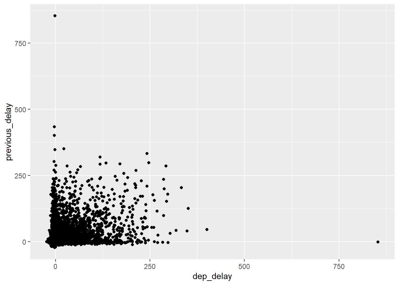
The resulting pattern remembers an arrow and is approximately the same for the other two origins (EWR and LGA) for each month. We can see that for increasing values of one axis the distribution of the values on the second axis decrease, and vice versa. This suggest that the an high delay for one flight tend to decrease for the next one.
Question 6: Look at each destination. Can you find flights that are suspiciously fast? (i.e. flights that represent a potential data entry error). Compute the air time of a flight relative to the shortest flight to that destination. Which flights were most delayed in the air?
The fastest flights are:
## # A tibble: 327,346 x 3
##    origin dest  air_time
##    <chr>  <chr>    <dbl>
##  1 EWR    BDL         20
##  2 EWR    BDL         20
##  3 EWR    BDL         21
##  4 EWR    PHL         21
##  5 EWR    BDL         21
##  6 EWR    PHL         21
##  7 LGA    BOS         21
##  8 JFK    PHL         21
##  9 EWR    BDL         21
## 10 EWR    BDL         21
## # ... with 327,336 more rows
While the flights that were the most delayed in the air are:
flights %>% filter(!is.na(air_time)) %>%
arrange(air_time) %>%
select(origin, dest, air_time) %>%
group_by (origin, dest) %>%
mutate(min_air_time = min(air_time), air_time_short_flight = air_time/min_air_time) %>%
arrange(desc(air_time_short_flight))
## # A tibble: 327,346 x 5
## # Groups: origin, dest [223]
## origin dest air_time min_air_time air_time_short_flight
## <chr> <chr> <dbl> <dbl> <dbl>
## 1 LGA BOS 107 21 5.10
## 2 LGA DCA 131 32 4.09
## 3 JFK ACK 141 35 4.03
## 4 EWR BOS 112 30 3.73
## 5 JFK BOS 96 26 3.69
## 6 LGA BOS 77 21 3.67
## 7 LGA BOS 76 21 3.62
## 8 LGA DCA 115 32 3.59
## 9 JFK BOS 91 26 3.5
## 10 LGA BOS 70 21 3.33
## # ... with 327,336 more rowsQuestion 7: Find all destinations that are flown by at least two carriers. Use that information to rank the carriers.
To find all destinations that are flown by at least two carriers with can use the following statement:
flights %>%
distinct(dest, carrier) %>%
group_by(dest) %>%
summarise(n()) %>%
filter(`n()` >= 2) %>%
arrange(desc(`n()`))
## # A tibble: 76 x 2
## dest `n()`
## <chr> <int>
## 1 ATL 7
## 2 BOS 7
## 3 CLT 7
## 4 ORD 7
## 5 TPA 7
## 6 AUS 6
## 7 DCA 6
## 8 DTW 6
## 9 IAD 6
## 10 MSP 6
## # ... with 66 more rowsThen the carriers’ ranking can be obtained by:
dest_2_carriers <- flights %>%
distinct(dest, carrier) %>%
group_by(dest) %>%
summarise(n()) %>%
filter(`n()` >= 2) %>%
arrange(desc(`n()`)) %>%
select(dest)

flights %>% filter(dest %in% dest_2_carriers$dest) %>%
distinct(carrier, dest)%>%
group_by(carrier) %>%
summarise(no_destinations = n()) %>%
arrange(desc(no_destinations))
## # A tibble: 16 x 2
## carrier no_destinations
## <chr> <int>
## 1 EV 51
## 2 9E 48
## 3 UA 42
## 4 DL 39
## 5 B6 35
## 6 AA 19
## 7 MQ 19
## 8 WN 10
## 9 OO 5
## 10 US 5
## 11 VX 4
## 12 YV 3
## 13 FL 2
## 14 AS 1
## 15 F9 1
## 16 HA 1Question 8: For each plane, count the number of flights before the first delay of greater than 1 hour.
What we should do is select all the flights ordered by tailnum and day and extract their delay. Then sum up all the delays value in a cumulative form and pick only the flights for which the cumulative sum in less than 1 hour (60 minutes).
Let’s take an example by considering the tail number N656UA:
flights %>% arrange(tailnum, month, day, dep_delay) %>%
filter(tailnum=='N656UA') %>% select(tailnum, dep_delay) %>%
mutate(cumsum_delays = cumsum(dep_delay), bool_cumsum_delays = cumsum(dep_delay) < 60)
## # A tibble: 5 x 4
## tailnum dep_delay cumsum_delays bool_cumsum_delays
## <chr> <dbl> <dbl> <lgl>
## 1 N656UA 14 14 TRUE
## 2 N656UA -2 12 TRUE
## 3 N656UA -7 5 TRUE
## 4 N656UA -1 4 TRUE
## 5 N656UA -3 1 TRUEThe previous statement shows that the single flight delay (dep_delay), the cumulative delay (cumsum_delays) and the boolean condition who checks the record that exceeds 60 minutes (bool_cumsum_delays). For the tail number N656UA we have 5 flights with the following delays in minutes: 14,-2,-7,-1,-3. Therefore the cumulative sum for the first flight is 14, for the second 14-2=12, for the third 14-2-7=5, for the fourth 14-2-7-1=4 and finally for the fifth 14-2-7-1-3=1. In this case the cumulative sum is under 60 minutes and we count no flights before the total delay exceeds 60 minutes.
Let’s take another example by considering the tail number N398SW:
flights %>% arrange(tailnum, month, day, dep_delay) %>%
filter(tailnum=='N398SW') %>% select(tailnum, dep_delay) %>%
mutate(cumsum_delays = cumsum(dep_delay), bool_cumsum_delays = cumsum(dep_delay) < 60)
## # A tibble: 6 x 4
## tailnum dep_delay cumsum_delays bool_cumsum_delays
## <chr> <dbl> <dbl> <lgl>
## 1 N398SW -2 -2 TRUE
## 2 N398SW 32 30 TRUE
## 3 N398SW 0 30 TRUE
## 4 N398SW -1 29 TRUE
## 5 N398SW 43 72 FALSE
## 6 N398SW -2 70 FALSENow we have 6 flights with the following delays in minutes: -2,32,0,-1,43,-2. Therefore the cumulative sum for the first flight is -2, for the second -2+32=30, for the third -2+32+0=30, for the fourth -2+32+0-1=29, for the fifth -2+32+0-1+43=72. and finally for the sixth -2+32+0-1+43-2=70. In this case the cumulative sum is over 60 minutes and we see, by looking at the bool_cumsum_delays, that there are 4 flights before the total delay exceeds 60 minutes. The delay of the fifth flights is responsible for the switch.
Once we have this mechanism we can complete the code to find for all flights the number of flights before the first delay of greater than 1 hour.
flights %>% arrange(tailnum, month, day, dep_delay) %>%
select(tailnum, dep_delay) %>%
group_by(tailnum) %>%
mutate(cumsum_delays = cumsum(dep_delay), bool_cumsum_delays = cumsum(dep_delay) < 60) %>%
filter(bool_cumsum_delays == 'TRUE') %>%
group_by(tailnum) %>%
summarise(n_of_flights = n())
## # A tibble: 3,793 x 2
## tailnum n_of_flights
## <chr> <int>
## 1 N0EGMQ 34
## 2 N10156 2
## 3 N102UW 25
## 4 N103US 46
## 5 N104UW 3
## 6 N105UW 27
## 7 N107US 38
## 8 N108UW 46
## 9 N109UW 48
## 10 N110UW 18
## # ... with 3,783 more rows